Kyle Karhohs
Imaging tissue slices provides a wealth of data about the spatial composition and number of the various cell types that make up a tissue. Interactions among cells within a tissue are crucial to understanding the role of the inflammation that is triggered by the invasion of cancerous cells. The strength of the inflammatory response has been linked to the prognosis of certain cancers such as lymphoma.
Quantifying the spatial relationship among cells in the crowded environment of a tissue requires reliable segmentation of several cell types. In lymph node sections, cells have representatives from the immune system, epithelial tissue, connective tissue, and cancer. Quantifying the cell locations provides the ability to gauge the degree to which the cancer has invaded a tissue and how the immune system is interacting with the leading edge of a tumor.
The ability to precisely measure this relationship will give a deeper understanding of the progression of cancer and might yield new insight into when and how the immune system is involved. Ultimately the aim is to define various configurations of this interaction that are predictive of patient outcome or the likelihood of success for a given treatment, such as immunotherapy.
CellProfiler and Tissue Data
In collaboration with the Margaret Shipp and Scott Rodig labs, we developed a pipeline in CellProfiler that addresses unique challenges presented by imaging tissue slices. Consider the image of a representative tissue slice (below), which reveals a field of view with a high cell density. The nuclei of all cells are stained (blue). Two cell types have been stained that are of particular interest in Hodgkin’s Lymphoma: Reed-Sternberg cells (aka RS in green), and tumor-associated macrophages (aka TAM in red).
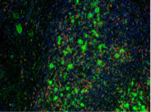
The greatest challenge in quantifying the spatial relationships among these cells, and the others surrounding them, is the identification of individual cell boundaries – a process known as segmentation. The density of the cells makes segmentation complicated as there is extensive overlapping between cell types, which is much greater than that seen even in dense monolayers of cultured cells. This overlapping stems from the fact that tissue slices reveal a plane from a 3D volume of cells from an excised portion of tissue. There are many cells that are not centered in this plane, i.e. their nuclei are not entirely captured within the slice. This increases the variety of nucleus size and intensity as some nuclei are only partially captured. Cytoplasmic regions of cells whose nuclei were not captured in the tissue slice can reside above or below fully captured nuclei; this increases the chance of mis-classifying cells. The positioning artifacts of nuclei described above are a complication to the analysis of a tissue image because most image analysis pipelines rely upon clear nucleus signal for seeding the segmentation of cytoplasmic regions.
In addition to the variety created by the mechanics of acquiring a tissue slice, tissue also contains more natural variety than cell lines. For example, RS cells are physically much larger than any of the neighboring cells. This size difference is a defining characteristic of this type of cell. Furthermore, other cells within a tissue have their own unique characteristics that add to the heterogeneity of size and shape. The two sources of variety mentioned thus far both complicate segmentation and quantification of the cells in a tissue slice.
We’ve developed a pipeline that addresses the challenges outlined above that are specific to tissue slices. The key innovation, as compared to pipelines that work well for monolayer cells, is prioritizing cell types based upon the quality of the marker and their size, and identifying them sequentially. Below is an overview of the method and pipeline:
1. IDENTIFY THE NUCLEI OF ALL CELLS:
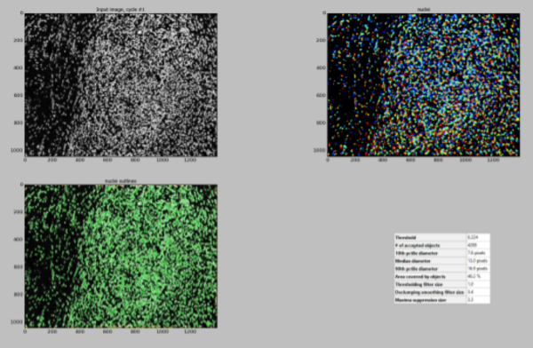
The nuclei can be identified from a nucleus stain such as DAPI. The segmentation of the nuclei will create a pool of “seeds”, or starting points, for the segmentation and classification of the various cell types within a tissue. Many of the nuclei will overlap, because the sectioning of a tissue captures cells through a volume. When a volume is projected into a 2D image, cells that are separated in Z will overlap. This can challenge segmentation of the nuclei. To improve results, the DAPI image is enhanced with a filter that strengthens the signal of round objects of a typical diameter using the EnhanceOrSuppressFeatures module.
2. CLASSIFY CELLS IN THE ORDER FROM MOST CERTAIN TO LEAST CERTAIN:
Prior knowledge of the tissue and cells within is imparted to the pipeline through the ordering of the segmentation steps. Stains with good signal and markers that strongly highlight a particular cell type are segmented with higher certainty in comparison to stains that are noisy or less-specific. In addition to the quality of staining, features and aspects unique to a cell type will also increase the certainty of segmentation when segmented objects of low certainty are removed using the FilterObjects module. In combination with the ordering of modules, the cells with the highest confidence are segmented before cells with lower confidence, and the segmentations of cells with higher confidence helps guide the segmentation of cells with lower confidence. In this example, we identify the HRS cells first because they are the largest and the stain for HRS cells also gives the strongest signal.
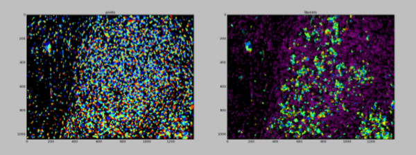
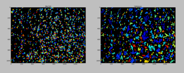
HRS cells’ nuclei are often fragmented. Using the nuclei as seeds leads to a fragmented segmentation of any given HRS cell. This is to be expected, so these fragmented regions are then “glued” together. Any two fragments of an HRS cell that touch are assumed to come from the same cell. This strategy works well with this cell type, because the spacing between HRS cells is generally large.
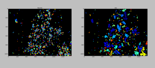
The same process is then used for TAM cells, which are also larger than average and have a strong staining signal.
3. ADDITIVE MASKING:
The remaining cells that are not already accounted for by the regions covered by the larger HRS and TAM cell types are then classified based upon the strength of their staining. To prevent double-counting the same cell as two different cell types (when appropriate, that is), a mask is created step by step that prevents the next cell types on the list from being identified in space already occupied by previously identified, more confident, cell types. First, candidate cells for a particular cell type are found by expanding the region defined as the nuclei to capture regions that include staining for the respective cell type.
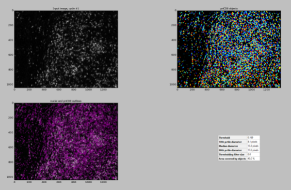
Then a mask, that is the sum of the areas occupied by upstream cell types, is applied to the candidate cells to remove those that have already been classified. What is left is then the cells that have gone unclaimed.
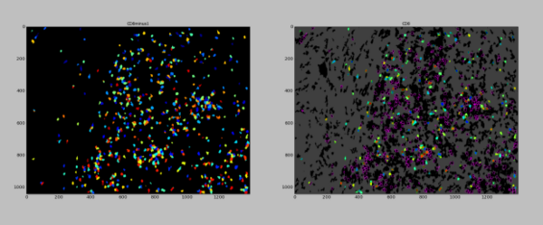
The mask grows after each round of segmentation, incorporating the cell types found before. After the final cell type has been segmented and classified, the remaining cells are segmented and classified as “unknown”.
Finally, the (x,y) location of each cell is exported to a spreadsheet. This table of locations can be analyzed to describe the spatial relationship among cells using downstream software applications such as R or Matlab.
