Melissa Gillis
In the first part of this blogpost I described some of the tools I tried to accurately segment collagen IV fibers including, CellProfiler, Cellpose, and Piximi. Unfortunately none of these methods were successful in accurately segmenting the fibers so I decided to develop a machine learning model in ilastik. In this section I will give an in depth explanation of how I created a successful segmentation model using ilastik.
Ilastik is a machine learning pixel classification and segmentation tool that is designed for individuals that don’t have an extensive background in machine learning. Ilastik doesn't require any coding to train a model, instead it prompts the user to hand annotate portions of their images, and then segments the remainder of the image based on these annotations. To train a model in ilastik, I first selected several representative images from the dataset that represented the full spectrum of variance in the data. It is important to note that when importing images into ilastik there are three main options for storing the images: absolute path, relative path, and copy into project file (image shown below).
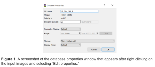
It is best practice to have the folder of training images stored in the same directory as the ilastik project file to make relative pathing easier. This will ensure that ilastik can always recognize the training images if they are within the same folder as the project file itself and makes it easier to share the model with someone else working on a different machine and prevents confusion later.
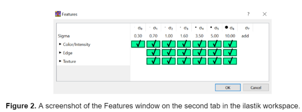
After I selected the input images, I selected the features for the model to consider on the second tab in the ilastik workspace. I selected all the available features, as this can improve the model's specificity and accuracy. The fibers I analyzed in these images were small, so the default features in ilastik proved sufficient. However, if segmenting larger objects I would recommend adding larger features to the existing list using the ‘add’ option to ensure that the true shape of the object is being detected.
After completing these preliminary steps, I moved on to training the images. I tried a variety of annotation styles and training options in ilastik to determine the best model for segmenting the fibers. In my first attempt, I tried annotating a wide variety of images from both Pearl’s original image set as well as the newer images. I originally decided to use 2 different classes or labels, blue for the background and yellow for the fibers. I decided to annotate the bright debris present in some of the original images as background in the hopes of differentiating them from the fibers. I attempted to mimic the general shape of the object while annotating, so drawing lines over fibers instead of annotating single pixels (see below).
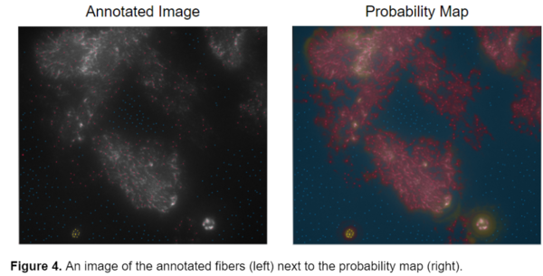
This resulted in probability maps that were unclear and identified the general region where the fibers were located but failed to accurately segment them individually, and had difficulty detecting the dimmer regions of fibers. This led me to explore a different approach.
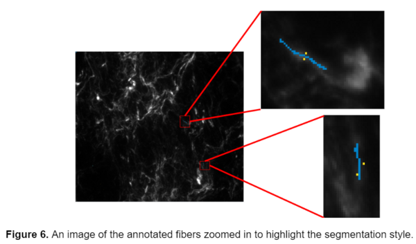
Instead of drawing the general outline of the objects in the image, I annotated single pixels on the fibers and tried to add as many points as possible in the hopes of attaining a better model. I also started using a three class model instead of the previous two class model where: red was for the collagen fibers, yellow was for the bright debris present in some of the original images, and blue was for the background . An example of this type of annotation is shown below.
This segmentation style was better, however, I still wanted to attain a more accurate segmentation of the fibers, so I looked at the uncertainty map from one of my previously annotated images to assess where failures could have originated from. The uncertainty map in ilastik displays how confident the program is in its segmentation. Bright blue areas represent regions where ilastik is unsure whether it should classify as fiber or background.
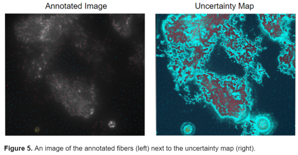
The model seemed to have the greatest uncertainty on the border between the fibers and the background. I realized that while I was placing a lot of points all over the image in the hopes of getting the best possible segmentation, I wasn’t placing the points in the most meaningful places, at the borders of fiber and background. I then realized that it wasn’t the sheer number of points that was crucial to the segmentation but their placement. All the uncertainty was coming from areas where the fibers meet the background. By turning on the uncertainty map before annotating the image I was able to identify the portions of the image that ilastik wasn’t sure about and increase annotations there. I then started annotating the image more concisely and very accurately, zooming in on individual fibers and carefully labeling the fibers as well as the pixels adjacent to them as the background. This greatly improved the accuracy and quality of the probability maps that ilastik produced.
While this segmentation style seemed to be working better it still wasn’t as accurate as I would have hoped for. ilastik seemed to be having difficulty distinguishing the yellow and red labels, for the bright debris and fibers respectively, from one another. It was inaccurately labeling some fibers as debris and debris as fibers, as seen in the above image. Because ilastik determines most of its segmentation based on intensity, it was very difficult for it to distinguish between the deris and some of the brighter fibers. I began thinking of ways to improve the model and decided to try annotating just the newer data without the bright debris, to eliminate the confusion and return back to a two class model. While ideally, I wanted the model to be able to work across a variety of fiber types, the two different types of images were so drastically different in terms of contrast, fiber composition, and density that I thought it would be best to create separate models for them. An example of the annotation style used in the final model is shown below, with background annotated in yellow and the fibers in blue.
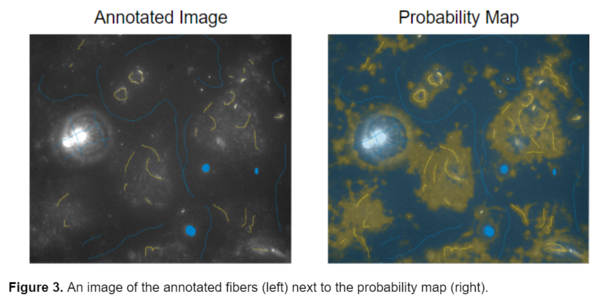
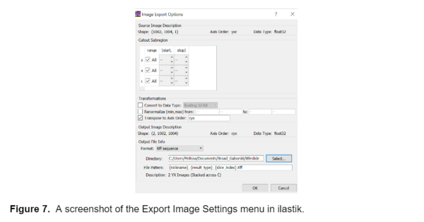
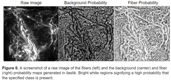
I used the trained model to segment the remainder of my data and retrained the model several times using images that represented poor segmentation to improve the model. Once I was happy with the model I uploaded all the images into ilastik and generated two probability maps, one for the background and one for the fibers, for each image. I exported these probability maps into a separate folder as tiff sequence files using the “4. Prediction Export” tab in ilastik, a screenshot of the export image settings menu is shown below, as well as an example of the probability maps.
Now that I had successfully segmented the fibers, I could use the probability maps generated from ilastik to perform measurements on the images. In the next section of this blogpost I will explain the CellProfiler pipeline I constructed to analyze the fibers.
Customizing a Model for Fiber Segmentation Series:
Part I: Investigating Possible Methods
Part 2: Creating an ilastik Model
Part 3: Constructing a CellProfiler Pipeline
Part 4: Analyzing the Results