
Pearl V. Ryder
In the previous post in this “Thinking like an image analyst” series, I explained how I enhanced fibers to increase their brightness and applied a background subtraction to decrease the intensity of the background. In combination with masking out very bright debris pixels (Part II of this series), these steps helped prepare this image for segmentation of the fibrils. If you’d like to follow along in CellProfiler, the pipeline and images for this project are available here.
In this post, I’ll explain how I detected the fibrils as individual objects using IdentifyPrimaryObjects. Once I identify the fibrils as objects, I can then measure many different attributes such as area, length, width, etc.
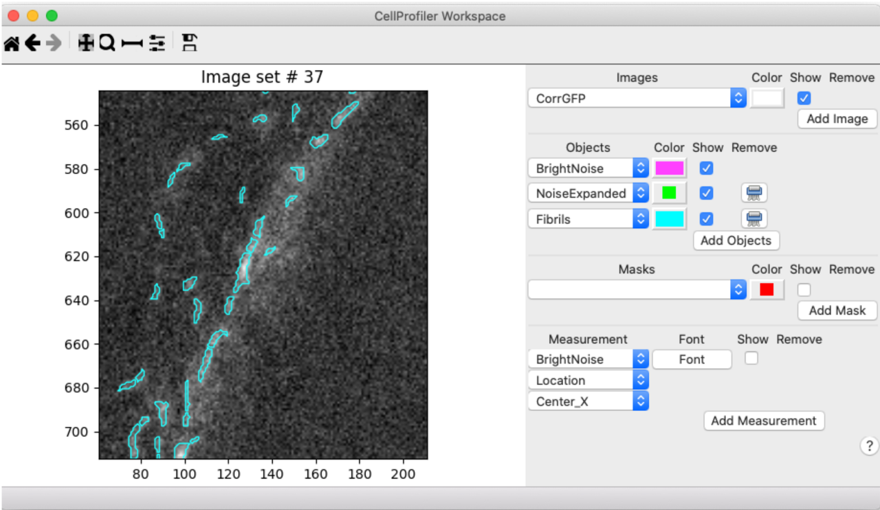
Since most of the image that we’re segmenting is background, I started by testing the Robust Background method for segmentation. See this blog post for an explanation of how the Robust Background method works. Happily, the default settings worked well for thresholding fibers. Since the image that we’re segmenting on has been enhanced and masked, I used the Workspace viewer to assess the segmentation while looking at the raw image to make sure my preprocessing steps hadn’t added or removed any “real” signal:
While I was happy with the thresholding of fibril vs. background, I noted that many of the longer fibrils were oversegmented (broken into too many pieces). In order to avoid this oversegmentation, I set the smoothing filter and the minimum distance between local maxima manually, an adjustment we often need to make for fibrillar structures (see the module help settings or our video on how exactly segmentation works in CellProfiler for more information). I chose values of 30 for each, which greatly improved the segmentation results, as you can see in this comparison:
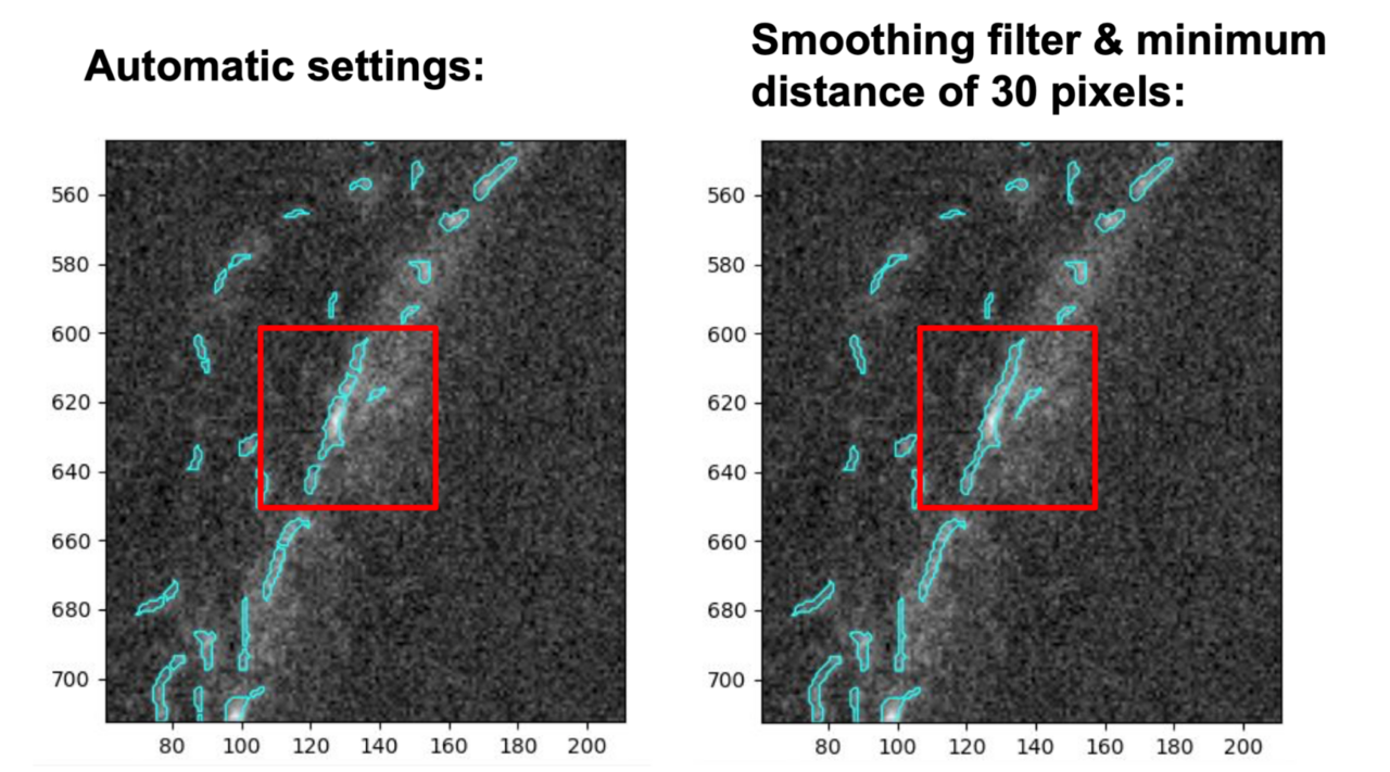
Comparison of the automatic settings for declumping (left) vs. manually setting the smoothing filter and minimum distance between local peaks to 30 pixels (right). If you focus on the objects within the red boxes, you can see how setting the smoothing filter and minimum distance manually reduced oversegmentation.
After examining this segmentation procedure on multiple images, I was happy with the segmentation results. I next added an OverlayObjects module to create an image with the fibril objects overlaid on top of the raw data. I then added a SaveImages module to automatically save these overlay images during each analysis run. This approach allows others to visualize the results of the segmentation and provides a record that can be reviewed later along with the data to verify results. It’s also a quick way to assess your segmentation results across all images (depending on the size of your dataset!).
Cropping out the image edges
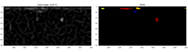
After running the segmentation on multiple images, I noted a common problem: many “fibrils” were detected in a horizontal line at the top of the image that probably weren’t real. I had a suspicion that this resulted as an artifact from the EnhanceOrSuppressFeatures module that I described in Part III. Sure enough, I could see an enhanced horizontal line of pixels at the top of the image that were within 10 pixels of the edge (these pixels weren’t bright in the original image):
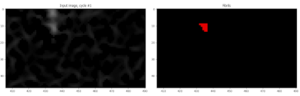
In order to get around this, I applied the Crop module to eliminate 10 pixels from the edges of the image. I used the rectangle mode of Crop w/ “from edge” mode selected. The resulting image no longer has the bright line enhanced at the top of the image and fibrils aren’t detected as a line at the top of the image. Voila!:
At this stage, we’ve successfully segmented our objects of interest. In the next and final post, I’ll describe how I finalized the pipeline by adding measurement modules and exporting the data.